I. Introduction
Let us figure out the effectiveness of whether detecting cancer by applying the k-NN algorithm to measurements of biopsied cells from women with abnormal breast masses. The dataset, "Wisconsin Breast Cancer Diagnostic" can be found from the UCI Machine Learning Repository. Browse through the area untill you see "Breast Cancer Wisconsin (Diagnostic) Data Set" on the right hand side. Click on the data folder and download "wdbc.data". This if the file we will be working with. If you would like a better explanation of the dataset and variables please click the "Data Description" tab. The dataset contains 569 observations, with 32 attributes. The first 12 contain Patient ID, cancer type and then:
- Radius
- Texture
- Perimeter
- Area
- Smoothness
- Compactness
- Concavity
- Concave points
- Symmetry
- Fractal dimension
The later attributes are just variants of the preceeding 10, such as Radius_StandardError or Radius Worst.
II. Exploring and Transforming the Dataset
The first step would be to import the data. You may import the data using the 'Import Dataset' button if you have RStudio installed, or use the following code:
> wbcd <- read.csv("wisc_bc_data.csv", stringsAsFactors = FALSE)
I suggest renaming the dataset afterwards, to ease out complex issues that may arise when you are trying to tell the variables a part. In order to this we will use the colnames() function. To understand the data and variables better, consider looking through the file data description in the same place you found the data. I have renamed this dataset using the data descriptions found.
colnames(wbcd) <-c("ID","diagnosis","radius_mean","texture_mean","perimeter_mean","area_mean","
smoothness_mean","compactness_mean","concavity_mean","concavepnts_mean","symmetry_mean",
"fractal_mean","radius_SE","texture_SE","perimeter_SE","area_SE","smoothness_SE","compactness_SE",
"concavity_SE","concavepts_SE","symmetry_SE","fractal_SE","vradiuse_worst","texture_worst",
"perimeter_worst","area_worst","smoothness_worst","compactness_worst","concavity_worst",
"concave_worst","symmetry_worst","fractal_worst")
If you have done everything correctly you should see that your data fram has 569 obs. of 32 varaibles. As we don't need the 'ID' for this problem, we can decide to drop it.
wbcd <- wbcd[-1]
Many R machine learning classifiers require that the target feature is coded as a factor, so we will need to recode the diagnosis variable.
> wbcd$diagnosis<- factor(wbcd$diagnosis, levels = c("B", "M"),
labels = c("Benign", "Malignant"))
Observing the prop.table() output,
> round(prop.table(table(wbcd$diagnosis)) * 100, digits = 1)
Benign Malignant
62.7 37.3
In order for us to apply this algorithm, we need to make sure that the variables do not significantly differ in size or else our results will tend to be inaccurate or biased. Therefore, it is always a good habbit to just check a statistical summary of the data. To take note of some statistical summaries we can use,
> summary(wbcd[c("radius_mean", "area_mean", "smoothness_mean")])
Observing above, we see that the Max for area_mean is 2501 which is drastically different. This calls us to normalize the data which we can write, apply and view by:
> normalize <- function(x) {
return ((x - min(x)) / (max(x) - min(x)))
}
> wbcd_n <- as.data.frame(lapply(wbcd[2:31], normalize))
> summary(wbcd_n$area_mean)
III. Training the dataset and Model
As we dont have access to new data, we cannot use the model to predict incoming data(from labs etc). Therefore, we must make use of what we have. Hence, we can split the dataset we have into 2 parts, one for training the dataset and the other one to verify how well we have trained the last dataset. If trained correctly, the model from the first dataset should be able to accurately guess the diagnostics of the observations from the second dataset. We will use 469 observations to train the first set, and 100 observations to verify. We can split the dataset by using:
> wbcd_train <- wbcd_n[1:469, ]
> wbcd_test <- wbcd_n[470:569, ]
When we constructed our normalized training and test datasets, we excluded the target variable, diagnosis. For training the k-NN model, we will need to store these class labels in factor vectors, split between the training and test datasets:
> wbcd_train_labels <- wbcd[1:469, 1]
> wbcd_test_labels <- wbcd[470:569, 1]
In order to continue building our model, we will need a package called "class". Install and load it using:
> install.packages("class")
> library(class)
IV. Applying the KN-Algorithm and Testing
We can finally apply the alogrithm and cross check the results to see how we did. We can choose the value of k=21(as its the closest to the sq.rt of 469). We can use the following formula
> wbcd_test_pred <- knn(train = wbcd_train, test = wbcd_test, cl = wbcd_train_labels, k = 21)
It will yield a result similar to this
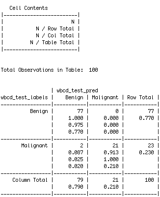
The cell percentages in the table indicate the proportion of values that fall into four categories. The top-left cell indicates the true negative results. These 77 of the 100 values are the trials where the diagnosis were benign and the k-NN algorithm correctly identified it! The bottom-right cell indicates the true positive results, where the algorithm predicted correctly again. A total of 21 of 100 predictions were true positives. This means that out of 100, our algorithm was able to predict 98 timees correctly.
The cells falling on the other diagonal contain counts of examples where the k-NN approach disagreed with the actual diagnosis. The two examples in the lower-left cell are false negative results; in this case, the predicted value was benign, but the tumor was actually malignant. This is the most dangerous cell block to have an error in, as it can wrongly diagnose a patient and make them believe they dont have cancer - where in turn, they do. The top-right cell would contain the false positive results, which we got as 0. These values occur when the model classifies a mass as malignant, but in reality, it was benign. These errors are less concerining, but could create drastic financial burden on patients who believe they have cancer, but dont and therefore are getting treated.
By carrying out the algorithm, we have a 98% accuracy. Applying this algorithm to new data would allow us to determine its accuracy better.